sankey
matplotlib.sankey
Module for creating Sankey diagrams using matplotlib
-
class matplotlib.sankey.Sankey(ax=None, scale=1.0, unit='', format='%G', gap=0.25, radius=0.1, shoulder=0.03, offset=0.15, head_angle=100, margin=0.4, tolerance=1e-06, **kwargs) -
Bases:
objectSankey diagram in matplotlib
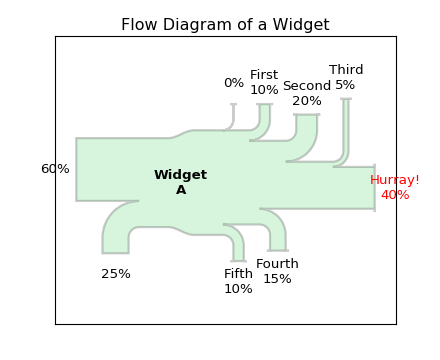
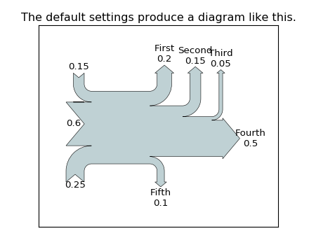
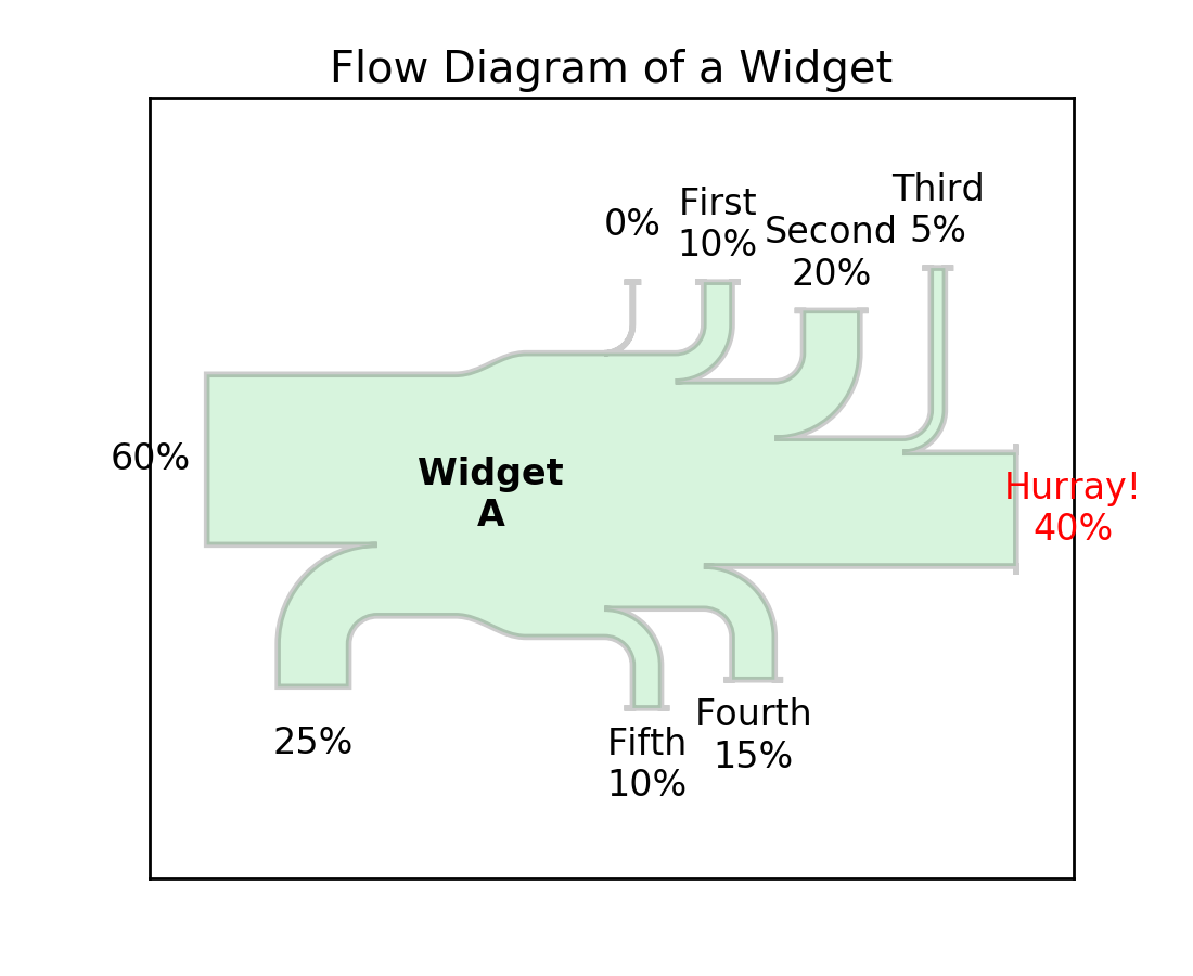
Sankey diagrams are a specific type of flow diagram, in which the width of the arrows is shown proportionally to the flow quantity. They are typically used to visualize energy or material or cost transfers between processes. Wikipedia (6/1/2011)Create a new Sankey instance.
Optional keyword arguments:
Field Description ax axes onto which the data should be plotted If ax isn’t provided, new axes will be created. scale scaling factor for the flows scale sizes the width of the paths in order to maintain proper layout. The same scale is applied to all subdiagrams. The value should be chosen such that the product of the scale and the sum of the inputs is approximately 1.0 (and the product of the scale and the sum of the outputs is approximately -1.0). unit string representing the physical unit associated with the flow quantities If unit is None, then none of the quantities are labeled. format a Python number formatting string to be used in labeling the flow as a quantity (i.e., a number times a unit, where the unit is given) gap space between paths that break in/break away to/from the top or bottom radius inner radius of the vertical paths shoulder size of the shoulders of output arrowS offset text offset (from the dip or tip of the arrow) head_angle angle of the arrow heads (and negative of the angle of the tails) [deg] margin minimum space between Sankey outlines and the edge of the plot area tolerance acceptable maximum of the magnitude of the sum of flows The magnitude of the sum of connected flows cannot be greater than tolerance. The optional arguments listed above are applied to all subdiagrams so that there is consistent alignment and formatting.
If
Sankeyis instantiated with any keyword arguments other than those explicitly listed above (**kwargs), they will be passed toadd(), which will create the first subdiagram.In order to draw a complex Sankey diagram, create an instance of
Sankeyby calling it without any kwargs:sankey = Sankey()
Then add simple Sankey sub-diagrams:
sankey.add() # 1
sankey.add() # 2
#...
sankey.add() # n
Finally, create the full diagram:
sankey.finish()
Or, instead, simply daisy-chain those calls:
Sankey().add().add... .add().finish()
Examples:
-
add(patchlabel='', flows=None, orientations=None, labels='', trunklength=1.0, pathlengths=0.25, prior=None, connect=(0, 0), rotation=0, **kwargs) -
Add a simple Sankey diagram with flows at the same hierarchical level.
Return value is the instance of
Sankey.Optional keyword arguments:
Keyword Description patchlabel label to be placed at the center of the diagram Note: label (not patchlabel) will be passed to the patch through **kwargsand can be used to create an entry in the legend.flows array of flow values By convention, inputs are positive and outputs are negative. orientations list of orientations of the paths Valid values are 1 (from/to the top), 0 (from/to the left or right), or -1 (from/to the bottom). If orientations == 0, inputs will break in from the left and outputs will break away to the right. labels list of specifications of the labels for the flows Each value may be None (no labels), ‘’ (just label the quantities), or a labeling string. If a single value is provided, it will be applied to all flows. If an entry is a non-empty string, then the quantity for the corresponding flow will be shown below the string. However, if the unit of the main diagram is None, then quantities are never shown, regardless of the value of this argument. trunklength length between the bases of the input and output groups pathlengths list of lengths of the arrows before break-in or after break-away If a single value is given, then it will be applied to the first (inside) paths on the top and bottom, and the length of all other arrows will be justified accordingly. The pathlengths are not applied to the horizontal inputs and outputs. prior index of the prior diagram to which this diagram should be connected connect a (prior, this) tuple indexing the flow of the prior diagram and the flow of this diagram which should be connected If this is the first diagram or prior is None, connect will be ignored. rotation angle of rotation of the diagram [deg] rotation is ignored if this diagram is connected to an existing one (using prior and connect). The interpretation of the orientations argument will be rotated accordingly (e.g., if rotation == 90, an orientations entry of 1 means to/from the left). Valid kwargs are
matplotlib.patches.PathPatch()arguments:Property Description agg_filterunknown alphafloat or None animated[True | False] antialiasedor aa[True | False] or None for default axesan Axesinstancecapstyle[‘butt’ | ‘round’ | ‘projecting’] clip_boxa matplotlib.transforms.Bboxinstanceclip_on[True | False] clip_path[ ( Path,Transform) |Patch| None ]colormatplotlib color spec containsa callable function edgecoloror ecmpl color spec, or None for default, or ‘none’ for no color facecoloror fcmpl color spec, or None for default, or ‘none’ for no color figurea matplotlib.figure.Figureinstancefill[True | False] gidan id string hatch[‘/’ | ‘\’ | ‘|’ | ‘-‘ | ‘+’ | ‘x’ | ‘o’ | ‘O’ | ‘.’ | ‘*’] joinstyle[‘miter’ | ‘round’ | ‘bevel’] labelstring or anything printable with ‘%s’ conversion. linestyleor ls[‘solid’ | ‘dashed’, ‘dashdot’, ‘dotted’ | (offset, on-off-dash-seq) | '-'|'--'|'-.'|':'|'None'|' '|'']linewidthor lwfloat or None for default path_effectsunknown picker[None|float|boolean|callable] rasterized[True | False | None] sketch_paramsunknown snapunknown transformTransforminstanceurla url string visible[True | False] zorderany number As examples,
fill=Falseandlabel='A legend entry'. By default,facecolor='#bfd1d4'(light blue) andlinewidth=0.5.The indexing parameters (prior and connect) are zero-based.
The flows are placed along the top of the diagram from the inside out in order of their index within the flows list or array. They are placed along the sides of the diagram from the top down and along the bottom from the outside in.
If the sum of the inputs and outputs is nonzero, the discrepancy will appear as a cubic Bezier curve along the top and bottom edges of the trunk.
See also
-
finish() -
Adjust the axes and return a list of information about the Sankey subdiagram(s).
Return value is a list of subdiagrams represented with the following fields:
Field Description patch Sankey outline (an instance of PathPatch)flows values of the flows (positive for input, negative for output) angles list of angles of the arrows [deg/90] For example, if the diagram has not been rotated, an input to the top side will have an angle of 3 (DOWN), and an output from the top side will have an angle of 1 (UP). If a flow has been skipped (because its magnitude is less than tolerance), then its angle will be None. tips array in which each row is an [x, y] pair indicating the positions of the tips (or “dips”) of the flow paths If the magnitude of a flow is less the tolerance for the instance of Sankey, the flow is skipped and its tip will be at the center of the diagram.text Textinstance for the label of the diagramtexts list of Textinstances for the labels of flowsSee also
-

© 2012–2016 Matplotlib Development Team. All rights reserved.
Licensed under the Matplotlib License Agreement.
http://matplotlib.org/1.5.3/api/sankey_api.html